- Introduction
In recent years a significant rise of cyberattacks has been detected1. The new normality derived from the COVID pandemic has led to an increase in the use of teleworking, as well as the use of more telematic processes that replace those previously carried out in person. This new lifestyle has become an attractive target for attackers, due to the fact that they have a large amount of information. In many cases this information is unprotected and with easily breakable access, which loss can provoke economical or even reputational damage. That is why cybersecurity has become such an important field in recent years.
One of the main factors which can help attackers to corrupt a system is the existence of vulnerabilities in the code. A simple vulnerability in the code can affect a whole system. Thus, it is vital to execute a suitable vulnerability assessment to the code.
To perform a good vulnerability and risk assessment process, it is important to complement a secure development methodology [1]. One of its main steps is to perform a code review or, in our case, the detection of critical or vulnerable code that can lead to a security breach. To this purpose, many have been the approaches used, having great relevance those focused on the use of Machine Learning (ML) and Data Mining (DM) algorithms. In the context of BIECO, we want to develop a tool which through ML and DM techniques is capable of detecting vulnerabilities within a static source code.
Detecting the existence of vulnerabilities within a system source is the first step in terms of vulnerability assessment. Nevertheless, such process alone is not enough to ensure a proper vulnerability assessment. Evaluating the severity or possible future impact of each discovered vulnerability are crucial steps when it comes to the security assessment in ICT components, as well as the prediction of future security threats for their risk identification. With it an improvement is achieved in order to prioritize mitigation efforts. Thus, and to provide the most comprehensive vulnerability assessment possible, three different forecasting tools are deployed. They are: a forecasting tool which estimates the likelihood of a given vulnerability to be exploited within a time window (e.g., 3, 6 or 12 months), a vulnerability forecasting tool which provides an estimation of the number of vulnerabilities to be expected in the main system software components for certain times frames, and a severity forecasting tool which predicts the severity of newly discovered and related vulnerabilities.
1.1. Connection with other tasks
The main purpose of WP3 is the research and development of the security tools and methodologies of BIECO’s framework that are oriented to risk and security assessment. Particularly, it is focused on the detection, forecasting and propagation of vulnerabilities across complex ICT systems.
In the case of the task T3.3, four different tools are deployed to be implemented within the design phase: one focused on the detection of vulnerabilities in the source code, and another three which forecast different parameters related with the vulnerabilities.
If we focus on those corresponding to task T3.3, it is possible to observe how these depend on vulnerability database (mostly from the Data Collection Tool developed in T3.2), as well as how their different outputs provide the input to the tools created in WP7 for the security claim evaluation.
For a better understanding of the tools aforementioned, the deliverable is organized as follows:
Section 2 introduces the vulnerability detection tool, focusing on the description of the process to acquire the dataset to be used for the training of the ML algorithms, a theoretical description of the different methods adopted in the process of evaluation as well as the reasons for their selection, and the implementation and obtained results of the different models trained.
Section 3 presents the three different forecasting tools developed within WP3: exploitability forecasting tool, vulnerability forecasting tool and a new severity forecasting tool, surged at the beginning of this task. In it, a description of each tool as well as the models considered for their implementation, possible features and results, if any, are provided. Due to the recent incorporation of the development of a severity forecasting tool, in this case, only the tool is presented offering a brief state of the art and possible algorithms to be used.
Section 4 concludes the deliverable by reporting the conclusions obtained in the tool development process as well as future actions to be taken.
Vulnerability Detection
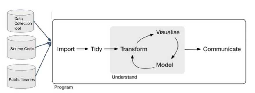
As it was mentioned in previous deliverables, [2] and [3], there are several procedures and techniques developed for the detection of vulnerabilities in the source code. After an extensive study and once the different existing possibilities have been assessed, a combination of techniques has been chosen boarding ML and DM techniques. In a first stage of the project, it has been decided to design a tool using Vulnerability Prediction Models (VPM) to detect vulnerable libraries in Python code. Detecting if a component could contain a vulnerability, helps to focus future efforts when analyzing the type of vulnerability contained. Once the approach has been chosen, it is necessary to obtain and transform the data to be used, following the steps of a typical data analytic project (Figure bellow).
For the development of the aforementioned techniques, the task has been divided in different phases:
- Obtention of the dataset to use for the analysis of the models, which includes the search for different public repositories of vulnerability datasets, its download or import, and its tidiness (Section 2.1),
- a transformation of the dataset to acquire the selection of the different features which characterize the inputs/outputs of the models,
- an analysis of different ML prediction models (Section 2.2),
- and the implementation and results obtained from those (Section 2.3).
2.1 Dataset
In order to obtain a public dataset for the training of ML algorithms, a library download tool has been created. This tool takes public libraries from Pypi repositories and divides them into vulnerable and not vulnerable. For having this classification, it has been consulted a repository that indicates which libraries and versions are vulnerable to a given CVE (Common Vulnerabilities and Exposures) or PVE, in case that the CVE is still provisional.
After parsing the repository, the data is processed to obtain extra information, such as the versions in a library that are not vulnerable or their corresponding CWE (Common Weakness Enumeration), if available, which will be used by further analysis. Once the data is processed a total of 3204 versions of different libraries have been downloaded. For a first phase of the evaluation, libraries and their versions are divided in two categories:
- vulnerable, that are those which have at least one known vulnerability, and
- safe, those that have no known vulnerabilities.
After having carried out this classification, 1930 vulnerable and 1274 not vulnerable libraries have been obtained. This division is going to characterize the analysis which will determine if a library is vulnerable or not.
2.1.1 Features
Once the data is provided, it is necessary to define the variables that will provide the necessary information to predict the existence or not of vulnerabilities. To this end, it is required a preprocessing of the acquired information. Data preprocessing is understood as the computation needed to transform the collected data into suitable input data for modeling. This procedure implies tidiness of the data by storing them in a consistent form which corresponds to the descriptive characteristics of the collected data, i.e., features. This transformation implies the creation of new variables of interest, to calculate a set of summary statistics, etc. These features are used as inputs to the ML models to characterize the problem to solve.
The obtention of the descriptive variables that will appear in the dataset is made by the use of different tools. These tools perform a static analysis of the source code and extract different characteristics such as the number of lines, possible dependencies with security issues or the complexity, among others. To acquire the features to be used in the ML models for the detection tool, different existing tools have been used, as well as an internal developed tool which will provide those features not able to be obtained by the existing ones.
Bandit (static code analysis)
Bandit is a tool which provides common security issues in Python code. To do this, it processes each file, acquiring its Abstract Syntactic Tree (AST), and runs different plugins against the AST nodes. Once the process is finished, Bandit generates a report, available in different formats, with different issues together with the number of evaluated lines in the code and the number of issues classified by confidentiality and severity. The features obtained are the following:
• Plugin tests: which encompasses misc. tests, application/framework misconfiguration, blacklists (calls and imports), cryptography, injection and XSS (Cross Site Scripting)
• Confidence: high, low, medium and undefined
• Severity: high, low medium and undefined
Radon
Radon is a tool based in Python which computes various code metrics to obtain information about code complexity. These supported metrics are:
• Raw metrics: based on the evaluation about the lines of the code. This information includes: LOC (lines of code), LLOC (logical lines of code), SLOC (source lines of code), comment lines and blank lines.
• Cyclomatic Complexity (i.e., McCabe’s Complexity): a quantitative measure of the logical complexity presented by a code calculated from the associated AST.
• Halstead metrics: focused on the different Python operators (arithmetic, logic, assign…) which can lead to the existence of bugs.
• Maintainability Index (a Visual Studio metric): a software metric to assess the level of difficulty to support or modify a code.
Safety (dependency check)
Safety is a command line tool that checks the local virtual environment, required files or any input from stdin for dependencies with security issues. As a result of the analysis, the tool provides a dependency report indicating those vulnerable libraries on which they are dependent on.
AST feature extractor tool
In addition to the previously described tools, an internal one has been developed to acquire those features of interest that the existing tools are not able to provide.
The tool, developed in Python, uses the public library ast to obtain the AST code representation. AST is an abstract representation of the source code that keeps the structural and context details, excluding all the inessential punctuation and
delimiters such as braces, semicolons or parentheses. This is often used by compilers as an intermediate representation before generating the binary executable since they can be modified and enhanced programmatically (e.g., to check the correctness of the syntax, remove death code or apply some high-level optimizations.) (detailed in Annex A)
In our case we use the AST to extract or calculate different features which will describe the static characteristics of the code such as the number lines, function classes or the imported libraries between others. Even though it is possible to obtain these features without the use of this representation, the extraction of the AST makes it easier and, in some cases, instantaneous.
In order to obtain the final dataset and given the heterogeneity of the downloaded files, it is necessary to perform certain adaptation tasks to the downloaded libraries for being able to use the different tools selected and, therefore, obtain the features in a standardized way. After processing the filtered data, a total of 2159 records (1398 vulnerable and 761 no vulnerable) and 144 different features have been evaluated.
2.2 Models
Once the different features have been obtained, they are analyzed through a training process using different ML metrics based on predictive models. These models are based on the use of a unique equation applied to an entire sample space. Occasionally, its implementation is hard due to the fact that it can result difficult to find a single global model capable of reflecting the relationship between the variables.
As previous works reviewed in the state of the art in [2], and taking into account the complexity of the calculated features and the results to be obtained, as starting point it has been chosen the tree-based method Random Forest (RF). Thinking ahead about the possibility of obtaining results that are not clarifying enough, three more models are implemented to provide a complete analysis and achieve the best results through their comparison. These models are Gradient Boosting Tree (GBT), Support Vector Machine (SVM) and Generalized Additive Models (GAM).
2.2.1 Tree-based methods
Tree-based methods have become one of the benchmarks within the predictive fields since they provide good results in different areas, either regression or classification problems [5]. These methods encompass a set of supervised techniques that are able to split an entire sample space into simple regions, which makes it easier to handle their interactions. To do so, an initial node is taken as the beginning, which is formed by the entire training sample, and subdivided conditioned by a certain feature into two new subsets, giving rise to two new nodes. This process is performed recursively with subsequent created nodes until a predetermined finite number of times, thus obtaining a final decision tree whose nodes are used to perform the prediction.
In the case of predicting if a certain library is vulnerable or not, the nodes generated by the tree-based method should be pure, that is, vulnerable or no vulnerable observations. Nevertheless, the fulfillment of this condition in practice is difficult to achieve, due to the nature of the available data. This results in models that, even though they have low bias, they present high variability, that is, a small data variation can lead to the creation of a different decision tree. Acquiring a balance between bias and variance is one of the main issues we can face when it comes to the selection of the tree-based model to use.
Random Forest
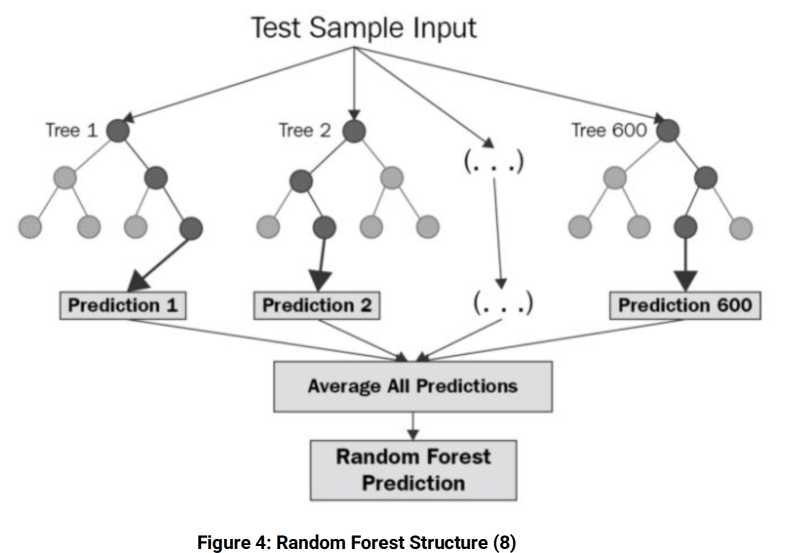
As discussed above, one of the main issues we can face when it comes to the use of tree-based methods, is to achieve a balance between bias and variance. To solve a possible decompensation between them, a combination of multiple models is used, better known as ensemble models, improving the predictions obtained by any of the original ones used individually. One of the most used ensemble models is bagging. These models adjust multiple models, each one trained with different training data, and provide the mean of the different obtained predictions or the most frequent class. One example of algorithm that is based on these models is Random Forest (RF) [5].
RF models offer suitable analysis results by implementing it in those scenarios in which a sheer number of features are handled. Some of the main advantages of such models are that they provide an automatic selection of predictors, which can be numerical or categorical, good scalability, low dependence on outliers and no need for standardization, among others.
This model is made up of an ensemble of individual decision trees which are trained individually with a random sample extracted from the original training data. The observations are distributed through the nodes generating the tree structure until reaching a terminal node or leaf. The set of predictions of each of the trees that make up the general model, generates the total prediction of the new observation.
Gradient Boosting Tree
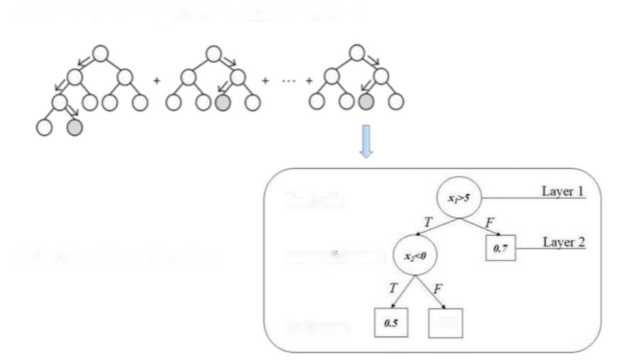
Another approach used to find the balance between bias and variance is the use of the ensemble models based on the use of boosting. Unlike bagging, these adjust sequentially multiple simple models. An example of these kind of models which use this kind of metric is Gradient Boosting Tree (GBT).
GBT are models made up of a set of individual decision trees, trained sequentially and achieving weak learners by the use of trees with one or few branches. Being run sequentially, each tree is trained by taking into account the information provided by the previous tree, correcting the prediction errors made to improve each iteration. This process is executed recursively until it achieves a final node, creating a complete tree structure. The prediction resulting from having executed all of them is the mean of all the individual results, or the most frequent class.
2.2.2 Support Vector Machine
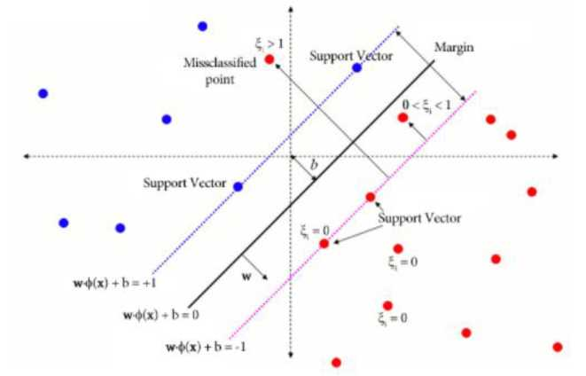
Another model to take into account is the use of the algorithm Support Vector Machine (SVM) [6]. This algorithm provides good results when it comes to datasets with binary classification outputs, which can suggest a good performance in the case of detecting the vulnerability or non-vulnerability of a library.
SVM is a supervised and linear ML algorithm that looks at data and sorts it into one of two categories. These types of methods were created to solve binary classification problems, based on the idea of dividing data through hyperplanes, and maintaining all the main features that characterize the algorithm.
2.2.3 Generalized Additive Models
An alternative methodology in terms of predictive models is the use of linear models, and in particular the General Linear Models (GLM) [7]. GLMs are a generalization of the stacking approach to ensemble learning that follows the concepts of the Super Learner models [8]. These models offer an approachable way to acquire a soft transition to more flexible models, while retaining some of the interpretability, as opposed to the opacity of many ML models.
To evaluate the possible improvement of results and make a more complete study, a model with a different approach was executed. In this case, it is decided to implement a model that allows greater flexibility in the dependence of each covariate with the response variable. This functionality can be obtained by the use of GLM which allows to interpret the features information knowledge. Nevertheless, despite the advantages offered by these kinds of models, they present some limitations when it comes to the relationship between predictors as well as the need for the variable response mean to be linear and constant. Thus, an extension of GLM which allows the use of non-linear relationships is used: GAM [9].
GAMs are regression models which require the assumption that the response variable follows a certain parametric distribution (normal, beta, and gamma), but with the particularity that the parameters used can be modeled, each one independently, following non-parametric functions (I.e., linear, additive or non-linear). This makes these models being considered as semi-parametric. Thanks to this versatility, GAMs are a suitable tool for the modeling of features which follow a wide range of distributions.
In these models, the relation between each predictor and splines.
The purpose of GAM is to maximize the prediction accuracy of a the variable response mean is not direct, but it is made through a function. The most used ones are the smooth non¬linear functions, such as cubic regression splines, tin plate regression splines or penalized dependent variable and several distributions, by specific non-parametric functions of the predictor variable which are connected to the dependent one through a link function.
2.3 Implementation and evaluation
When implementing ML tools, the selection of the input dataset for model training as well as the features to be used is crucial. For the implementation of the aforementioned methods, it is necessary to preprocess the acquired features through an Exploratory Data Analysis (EDA) from where different inferences can be drawn to ensure a selection of efficient features. After performing this EDA, it has been possible to verify a large presence of outlier data, as well as the existence of similar records, dependence between numerous features and low dependence of them with the response variable, among others. This assessment leads to the discarding of those features that could result in repetitions or that could have dependencies with others already calculated. After this preprocessing, a total of 84 features have been selected for the use of the models based on decision tree and the SVM.
Besides this filtering, algorithms based on logistic regression require a recompilation of features which are the most significant or provide the greatest contribution to the model. Thus, a selection has been carried out by discarding those variables with a high correlation between them. Furthermore, an own selection has been done taking those features which are considered the best significant option for a vulnerability prediction. After the analyses, a total of 48 features have been collected to be used in the model.
When it comes to the selection of the input dataset, and to avoid possible input data which could compromise the results, a balancing has been carried out, i.e., an approximately equal number of vulnerable and non-vulnerable samples have been selected. Likewise, and in order to make a complete evaluation of the models, two different scenarios have been created: one in which a set of paired data is provided, and another whose samples are unpair. For the former, a vulnerable and non-vulnerable version of each of the libraries has been chosen, while for the latter, the vulnerable and non-vulnerable samples correspond to different libraries. In the case of models GAM, the use of paired datasets does not provide satisfactory results, since they can lead to confusion. Therefore, the dataset used will be the one that, in addition to being balanced, has unpaired data.
To obtain the optimum results of the model, samples have been divided into those used for the training process and those used for testing. In addition, a grid search has been
implemented by cross validation for obtaining the hyperparameters corresponding to the best result of each model.
When implementing the different models, the use of the Python programming language has been chosen, since it includes specific libraries for performing their execution. In the case of RF, the public library RandomForestClassifier is used. GBT is implemented by the library GradientBoostingClassifier . SVM is configured by the use of the SVC from the public library sklearn . By last, for the implementation of linear generalized models two different methodologies have been applied: one based on the logistic regression model by the use of linear_model.LogisticRegression included in the Python library sklearn and another by implementing the generalization to the additive case of the linear model, using LogisticGAM() from the Python library sklearn.
The proportion between the records obtained and variables, together with the conclusions aforementioned and the exploratory nature of the study presented, favor the possibility of evaluating several different data sets. These are the result of performing certain transformations such as the grouping of certain variables, the elimination of paired data, the suppression of certain categorical variables, etc.
In a first test, it has been taken as a dataset those libraries vulnerable and no-vulnerable to a known CVE, that is, it has been discarded those libraries and versions marked with provisional CVE or PVE. The results obtained in the different models with said dataset are not conclusive since the number of existing samples in it is not enough for a correct implementation of the selected models.
To solve the lack of samples in the dataset, it has been taken those libraries with PVE, considering them as vulnerable, as well as their no-vulnerable version. These samples have been evaluated in both scenarios paired data and unpaired data, except for the GAM models which nature only allows their use with unpaired data.
| Scenario | Model | Accuracy training | Accuracy testing | AUC |
| Paired data | RF | 0.509 | 0.502 | 0.518 |
| GBT | 0.602 | 0.579 | 0.539 | |
| SVM | 0.6 | 0.581 | 0.541 | |
| Unpaired data | RF | 0.497 | 0.496 | 0.528 |
| GBT | 0.532 | 0.558 | 0.569 | |
| SVM | 0.552 | 0.554 | 0.552 | |
| GAM | 0.521 | 0.523 | 0.498 |
For the evaluation of the results, it has been taken into account the accuracy training, accuracy testing and the AUC (Area Under the ROC Curve) whose optimal values have to be around the 0.7 and 0.9. In this scenario, the obtained results (Table 1) showed low adjustments in all the models and scenarios indicating that a data extension has not
provided solutions in improving the modeling. When making a comparison between the different models and scenarios, there is no indication of a significant difference. In addition, having a low accuracy with the training data indicates that models are not being able to learn properly, which leads to consider performing an improvement of the problem context.
As a way of improvement of the model’s results, it has been chosen to add a contextualization on the dataset. For this, the possibility of adding new features to the existing ones has been evaluated, which can characterize more accurately the response feature of the same. After various analyses, a reconfiguration of the output feature is performed.
The results obtained after the execution of the models with the new reconfiguration are those shown in Table 2. Since the results obtained with the paired and unpaired data do not show any difference, only those whose dataset are paired are shown, but the GAM models which only allows their use with unpaired data.
| Model | Accuracy training | Accuracy testing | AUC |
| RF | 0.566 | 0.561 | 0.623 |
| GBT | 0.651 | 0.634 | 0.628 |
| SVM | 0.653 | 0.631 | 0.535 |
| GAM | 0.642 | 0.564 | 0.573 |
After the obtention of the results, it can be seen that, in general terms, all the models present a slight improvement after the response reconfiguration. Likewise, the trend in the variation within the training test settings is maintained. However, the differences between the models are still not significant, and the unpaired scenario presents a weaker improvement regarding this information.
During the process of reformulating the problem, the possibility of modifying the response feature is explored taking into account the different types of CVE contained in the libraries. Since a certain library can have several different vulnerabilities, the possibility of obtaining a new dataset is contemplated, in which the records corresponding to a certain library appear as many times as different CVEs contain.
In this way, a new dataset has been generated which includes all the original libraries considered no-vulnerable, and those vulnerable to a given CVE, discarding those with PVE label. Due to the fact that data samples are paired, GAM is not performed as its use confuses the model giving unsatisfactory results. This dataset contains a total of 1613 records.
| Model | Accuracy training | Accuracy testing | AUC |
| RF | 0.754 | 0.727 | 0.776 |
| GBT | 0.751 | 0.702 | 0.719 |
| SVM | 0.653 | 0.621 | 0.637 |
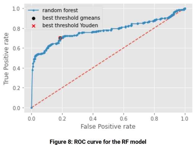
The execution of the algorithms with the new dataset provides results in which a significant improvement can be verified with respect to the previous one (Table 3). In this case, the evaluated models present an improvement in the adjustment reached around 75%, being the model RF the one that provides the best results. The evaluation of the performance of said model offers a confusion matrix with false positive and false negative rates greater than 10%.
In addition, the obtained report details other representative measures such as precision (number of true positives that are actually positive compared to the total number of predicted positive values), recall (number of true positives that the model has classified based on the total number of positive values) and F1 score (harmonic mean of the above) (Table 4), which values are around 70% in both precision and recall.
| Outputs | Precision | Recall | F1-score | % Support |
| 0 | 0.72 | 0.754 | 0.727 | 0.493 |
| 1 | 0.74 | 0.653 | 0.621 | 0.507 |
By focusing on the ROC curve (Figure 8) and the AUC, it is possible to observe a summary of the model’s performance, which is close to 80%.
As a result of the different transformations carried out to improve the evaluations, it has been verified that the results do not depend to a great extent on the chosen model, since they provide similar results between them. Moreover, adding records to the sample does not provide relevant improvements. Only by adding context to the problem and recoding the response feature provides slight improvements to the results.